Machine learning with missing values

Here we use simulated data to understanding the fundamentals of statistical learning with missing values.

This notebook reveals why a HistGradientBoostingRegressor ( sklearn.ensemble.HistGradientBoostingRegressor ) is a good choice to predict with missing values.

We use simulations to control the missing-value mechanism, and inspect it’s impact on predictive models. In particular, standard imputation procedures can reconstruct missing values without distortion only if the data is missing at random.

A good introduction to the mathematics behind this notebook can be found in https://arxiv.org/abs/1902.06931

Missing values in categorical data

If a categorical column has missing values, the simplest approach is to create a specific category “missing” and assign missing values to this new category, to represent missingness in the classifier. Indeed, as we will see, imputation is not crucial for prediction. In the following we focus on continuous columns, where the discrete nature of a missing value poses more problems.

The fully-observed data: a toy regression problem

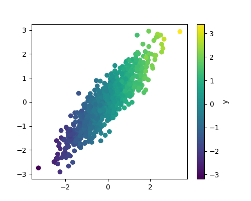
We consider a simple regression problem where X (the data) is bivariate gaussian, and y (the prediction target) is a linear function of the first coordinate, with noise.

The data-generating mechanism

import numpy as np

def generate_without_missing_values(n_samples, rng=42):
    mean = [0, 0]
    cov = [[1, 0.9], [0.9, 1]]
    if not isinstance(rng, np.random.RandomState):
        rng = np.random.RandomState(rng)
    X = rng.multivariate_normal(mean, cov, size=n_samples)

    epsilon = 0.1 * rng.randn(n_samples)
    y = X[:, 0] + epsilon

    return X, y

A quick plot reveals what the data looks like

import matplotlib.pyplot as plt
plt.rcParams['figure.figsize'] = (5, 4) # Smaller default figure size

plt.figure()
X_full, y_full = generate_without_missing_values(1000)
plt.scatter(X_full[:, 0], X_full[:, 1], c=y_full)
plt.colorbar(label='y')

<matplotlib.colorbar.Colorbar object at 0x7fd79d08b8d0>

Missing completely at random settings

We now consider missing completely at random settings (a special case of missing at random): the missingness is completely independent from the values.

The missing-values mechanism

def generate_mcar(n_samples, missing_rate=.5, rng=42):
    X, y = generate_without_missing_values(n_samples, rng=rng)
    if not isinstance(rng, np.random.RandomState):
        rng = np.random.RandomState(rng)

    M = rng.binomial(1, missing_rate, (n_samples, 2))
    np.putmask(X, M, np.nan)

    return X, y

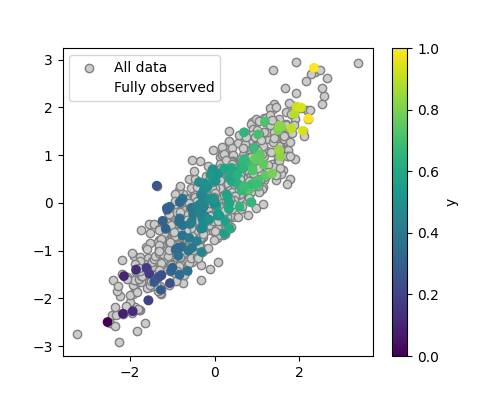
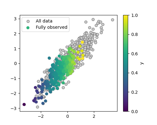
A quick plot to look at the data

X, y = generate_mcar(500)

plt.figure()
plt.scatter(X_full[:, 0], X_full[:, 1], color='.8', ec='.5', label='All data')
plt.colorbar(label='y')
plt.scatter(X[:, 0], X[:, 1], c=y, label='Fully observed')
plt.legend()

<matplotlib.legend.Legend object at 0x7fd79a391dd0>

We can see that the distribution of the fully-observed data is the same than that of the original data

Conditional Imputation with the IterativeImputer

As the data is MAR (missing at random), an imputer can use the conditional dependencies between the observed and the missing values to impute the missing values.

We’ll use the IterativeImputer, a good imputer, but it needs to be enabled

from sklearn.experimental import enable_iterative_imputer
from sklearn import impute
iterative_imputer = impute.IterativeImputer()

Let us try the imputer on the small data used to visualize

The imputation is learned by fitting the imputer on the data with missing values

iterative_imputer.fit(X)

IterativeImputer()

In a Jupyter environment, please rerun this cell to show the HTML representation or trust the notebook.
On GitHub, the HTML representation is unable to render, please try loading this page with nbviewer.org.

The data are imputed with the transform method

X_imputed = iterative_imputer.transform(X)

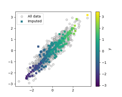
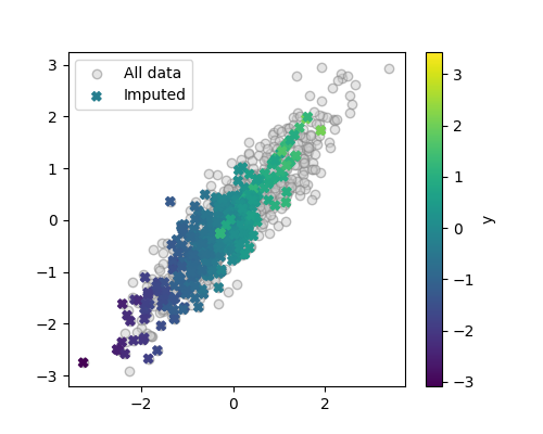
We can display the imputed data as our previous visualization

plt.figure()
plt.scatter(X_full[:, 0], X_full[:, 1], color='.8', ec='.5',
            label='All data', alpha=.5)
plt.scatter(X_imputed[:, 0], X_imputed[:, 1], c=y, marker='X',
            label='Imputed')
plt.colorbar(label='y')
plt.legend()

<matplotlib.legend.Legend object at 0x7fd79c1c1750>

We can see that the imputer did a fairly good job of recovering the data distribution

Supervised learning: imputation and a linear model

Given that the relationship between the fully-observed X and y is a linear relationship, it seems natural to use a linear model for prediction. It must be adapted to missing values using imputation.

To use it in supervised setting, we will pipeline it with a linear model, using a ridge, which is a good default linear model

from sklearn.pipeline import make_pipeline
from sklearn.linear_model import RidgeCV

iterative_and_ridge = make_pipeline(impute.IterativeImputer(), RidgeCV())

We can evaluate the model performance in a cross-validation loop (for better evaluation accuracy, we increase slightly the number of folds to 10)

from sklearn import model_selection
scores_iterative_and_ridge = model_selection.cross_val_score(
    iterative_and_ridge, X, y, cv=10)

scores_iterative_and_ridge

array([0.61639853, 0.5814862 , 0.70136887, 0.64571923, 0.58785589,
       0.79618649, 0.65278055, 0.8454113 , 0.81722841, 0.76948479])

Computational cost: One drawback of the IterativeImputer to keep in mind is that its computational cost can become prohibitive of large datasets (it has a bad computation scalability).

Mean imputation: SimpleImputer

We can try a simple imputer: imputation by the mean

mean_imputer = impute.SimpleImputer()

A quick visualization reveals a larger disortion of the distribution

X_imputed = mean_imputer.fit_transform(X)
plt.figure()
plt.scatter(X_full[:, 0], X_full[:, 1], color='.8', ec='.5',
            label='All data', alpha=.5)
plt.scatter(X_imputed[:, 0], X_imputed[:, 1], c=y, marker='X',
            label='Imputed')
plt.colorbar(label='y')

<matplotlib.colorbar.Colorbar object at 0x7fd757482a90>

Evaluating in prediction pipeline

mean_and_ridge = make_pipeline(impute.SimpleImputer(), RidgeCV())
scores_mean_and_ridge = model_selection.cross_val_score(
    mean_and_ridge, X, y, cv=10)

scores_mean_and_ridge

array([0.58596256, 0.55215184, 0.61081314, 0.55282029, 0.54053836,
       0.64325051, 0.60147921, 0.84188079, 0.68152965, 0.67441335])

Supervised learning without imputation

The HistGradientBoosting models are based on trees, which can be adapted to model directly missing values

from sklearn.experimental import enable_hist_gradient_boosting
from sklearn.ensemble import HistGradientBoostingRegressor
score_hist_gradient_boosting = model_selection.cross_val_score(
    HistGradientBoostingRegressor(), X, y, cv=10)

score_hist_gradient_boosting

/home/varoquau/dev/scikit-learn/sklearn/experimental/enable_hist_gradient_boosting.py:15: UserWarning: Since version 1.0, it is not needed to import enable_hist_gradient_boosting anymore. HistGradientBoostingClassifier and HistGradientBoostingRegressor are now stable and can be normally imported from sklearn.ensemble.
  warnings.warn(

array([0.61170698, 0.56911116, 0.635685  , 0.62752111, 0.58094569,
       0.71569692, 0.62359162, 0.83829684, 0.81283438, 0.74080482])

Recap: which pipeline predicts well on our small data?

Let’s plot the scores to see things better

import pandas as pd
import seaborn as sns

scores = pd.DataFrame({'Mean imputation + Ridge': scores_mean_and_ridge,
             'IterativeImputer + Ridge': scores_iterative_and_ridge,
             'HistGradientBoostingRegressor': score_hist_gradient_boosting,
    })

sns.boxplot(data=scores, orient='h')
plt.title('Prediction accuracy\n linear and small data\n'
          'Missing Completely at Random')
plt.tight_layout()

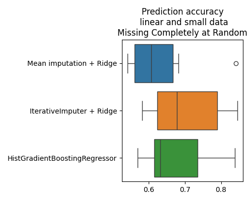
Not much difference with the more sophisticated imputer. A more thorough analysis would be necessary, with more cross-validation runs.

Prediction performance with large datasets

Let us compare models in regimes where there is plenty of data

X, y = generate_mcar(n_samples=20000)

Iterative imputation and linear model

scores_iterative_and_ridge= model_selection.cross_val_score(
    iterative_and_ridge, X, y, cv=10)

Mean imputation and linear model

scores_mean_and_ridge = model_selection.cross_val_score(
    mean_and_ridge, X, y, cv=10)

And now the HistGradientBoostingRegressor, which does not need imputation

score_hist_gradient_boosting = model_selection.cross_val_score(
    HistGradientBoostingRegressor(), X, y, cv=10)

We plot the results

scores = pd.DataFrame({'Mean imputation + Ridge': scores_mean_and_ridge,
             'IterativeImputer + Ridge': scores_iterative_and_ridge,
             'HistGradientBoostingRegressor': score_hist_gradient_boosting,
    })

sns.boxplot(data=scores, orient='h')
plt.title('Prediction accuracy\n linear and large data\n'
          'Missing Completely at Random')
plt.tight_layout()

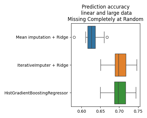
When there is a reasonnable amout of data, the HistGradientBoostingRegressor is the best strategy even for a linear data-generating mechanism, in MAR settings, which are settings favorable to imputation + linear model [1].

[1]

Even in the case of a linear data-generating mechanism, the optimal prediction one data imputed by a constant is a piecewise affine function with 2^d regions ( http://proceedings.mlr.press/v108/morvan20a.html ). The larger the dimensionality (number of features), the more a imperfect imputation is hard to approximate with a simple model.

Missing not at random: censoring

We now consider missing not at random settings, in particular self-masking or censoring, where large values are more likely to be missing.

The missing-values mechanism

def generate_censored(n_samples, missing_rate=.4, rng=42):
    X, y = generate_without_missing_values(n_samples, rng=rng)
    if not isinstance(rng, np.random.RandomState):
        rng = np.random.RandomState(rng)

    B = rng.binomial(1, 2 * missing_rate, (n_samples, 2))
    M = (X > 0.5) * B

    np.putmask(X, M, np.nan)

    return X, y

A quick plot to look at the data

X, y = generate_censored(500, missing_rate=.4)

plt.figure()
plt.scatter(X_full[:, 0], X_full[:, 1], color='.8', ec='.5',
            label='All data')
plt.colorbar(label='y')
plt.scatter(X[:, 0], X[:, 1], c=y, label='Fully observed')
plt.legend()

<matplotlib.legend.Legend object at 0x7fd754254e50>

Here the full-observed data does not reflect well at all the distribution of all the data

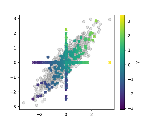
Imputation fails to recover the distribution

With MNAR data, off-the-shelf imputation methods do not recover the initial distribution:

iterative_imputer = impute.IterativeImputer()
X_imputed = iterative_imputer.fit_transform(X)

plt.figure()
plt.scatter(X_full[:, 0], X_full[:, 1], color='.8', ec='.5',
            label='All data', alpha=.5)
plt.scatter(X_imputed[:, 0], X_imputed[:, 1], c=y, marker='X',
            label='Imputed')
plt.colorbar(label='y')
plt.legend()

<matplotlib.legend.Legend object at 0x7fd7542d1c10>

Recovering the initial data distribution would need much more mass on the right and the top of the figure. The imputed data is shifted to lower values than the original data.

Note also that as imputed values typically have lower X values than their full-observed counterparts, the association between X and y is also distorted. This is visible as the imputed values appear as lighter diagonal lines.

An important consequence is that the link between imputed X and y is no longer linear, although the original data-generating mechanism is linear [2]. For this reason, it is often a good idea to use non-linear learners in the presence of missing values.

[2]

As mentionned above, even in the case of a linear data-generating mechanism, imperfect imputation leads to complex functions to link to y ( http://proceedings.mlr.press/v108/morvan20a.html )

Predictive pipelines

Let us now evaluate predictive pipelines

scores = dict()

# Iterative imputation and linear model
scores['IterativeImputer + Ridge'] = model_selection.cross_val_score(
    iterative_and_ridge, X, y, cv=10)

# Mean imputation and linear model
scores['Mean imputation + Ridge'] = model_selection.cross_val_score(
    mean_and_ridge, X, y, cv=10)

# IterativeImputer and non-linear model
iterative_and_gb = make_pipeline(impute.SimpleImputer(),
                            HistGradientBoostingRegressor())
scores['Mean imputation\n+ HistGradientBoostingRegressor'] = model_selection.cross_val_score(
    iterative_and_gb, X, y, cv=10)

# Mean imputation and non-linear model
mean_and_gb = make_pipeline(impute.SimpleImputer(),
                            HistGradientBoostingRegressor())
scores['IterativeImputer\n+ HistGradientBoostingRegressor'] = model_selection.cross_val_score(
    mean_and_gb, X, y, cv=10)

# And now the HistGradientBoostingRegressor, whithout imputation
scores['HistGradientBoostingRegressor'] = model_selection.cross_val_score(
    HistGradientBoostingRegressor(), X, y, cv=10)

# We plot the results
sns.boxplot(data=pd.DataFrame(scores), orient='h')
plt.title('Prediction accuracy\n linear and small data\n'
          'Missing not at Random')
plt.tight_layout()

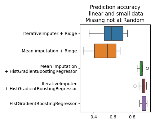
We can see that the imputation is not the most important step of the pipeline [3], rather what is important is to use a powerful model. Here there is information in missingness (if a value is missing, it is large), information that a model can use to predict better.

[3]

Note that there are less missing values in the example here compared to the section above on MCAR, hence the absolute prediction accuracies are not comparable.

Prediction with missing values

The data above are very simple: linear data-generating mechanism, Gaussian, and low dimensional. Yet, they show the importance of using non-linear models, in particular the HistGradientBoostingRegressor which natively deals with missing values.

Using a predictor for the fully-observed case

Let us go back to the “easy” case of the missing completely at random settings with plenty of data

n_samples = 20000

X, y = generate_mcar(n_samples, missing_rate=.5)

Suppose we have been able to train a predictive model that works on fully-observed data:

X_full, y_full = generate_without_missing_values(n_samples)
full_data_predictor = HistGradientBoostingRegressor()
full_data_predictor.fit(X_full, y_full)

model_selection.cross_val_score(full_data_predictor, X_full, y_full)

array([0.98934188, 0.9897668 , 0.98932951, 0.98916616, 0.98898611])

The cross validation reveals that the predictor achieves an excellent explained variance; it is a near-perfect predictor on fully observed data

Now we turn to data with missing values. Given that our data is MAR (missing at random), we will use imputation to build a completed data that looks like the full-observed data

iterative_imputer = impute.IterativeImputer()
X_imputed = iterative_imputer.fit_transform(X)

The full data predictor can be used on the imputed data

from sklearn import metrics
metrics.r2_score(y, full_data_predictor.predict(X_imputed))

0.7011318399077224

This prediction is less good than on the full data, but this is expected, as missing values lead to a loss of information. We can compare it to a model trained to predict on data with missing values

X_train, y_train = generate_mcar(n_samples, missing_rate=.5)
na_predictor = HistGradientBoostingRegressor()
na_predictor.fit(X_train, y_train)

metrics.r2_score(y, na_predictor.predict(X))

0.7036144866135492

Applying a model valid on the full data to imputed data work almost as well as a model trained for missing values. The small loss in performance is because the imputation is imperfect.

When the data-generation is non linear

We now modify a bit the example above to consider the situation where y is a non-linear function of X

X, y = generate_mcar(n_samples, missing_rate=.5)
y = y ** 2

# Train a predictive model that works on fully-observed data:
X_full, y_full = generate_without_missing_values(n_samples)
y_full = y_full ** 2
full_data_predictor = HistGradientBoostingRegressor()
full_data_predictor.fit(X_full, y_full)

model_selection.cross_val_score(full_data_predictor, X_full, y_full)

array([0.97018219, 0.96754963, 0.96600898, 0.96971664, 0.96795887])

Once again, we have a near-perfect predictor on fully-observed data

On data with missing values:

iterative_imputer = impute.IterativeImputer()
X_imputed = iterative_imputer.fit_transform(X)

from sklearn import metrics
metrics.r2_score(y, full_data_predictor.predict(X_imputed))

0.5330009632809711

The full-data predictor works much less well

Now we use a model trained to predict on data with missing values

X_train, y_train = generate_mcar(n_samples, missing_rate=.5)
y_train = y_train ** 2
na_predictor = HistGradientBoostingRegressor()
na_predictor.fit(X_train, y_train)

metrics.r2_score(y, na_predictor.predict(X))

0.657124508956336

The model trained on data with missing values works significantly better than that was optimal for the fully-observed data.

Only for linear mechanism is the model on full data also optimal for perfectly imputed data. When the function linking X to y has curvature, this curvature turns uncertainty resulting from missingness into bias [4].

[4]

The detailed mathematical analysis of prediction after imputation can be found here: https://arxiv.org/abs/2106.00311

---