
Note
Go to the end to download the full example code. or to run this example in your browser via JupyterLite or Binder
Dirty categories: learning with non normalized strings
Including strings that represent categories often calls for much data preparation. In particular categories may appear with many morphological variants, when they have been manually input, or assembled from diverse sources.
Including such a column in a learning pipeline as a standard categorical colum leads to categories with very high cardinalities and can lose information on which categories are similar.
Here we look at a dataset on wages [1] where the column Employee Position Title contains dirty categories.
We investigate encodings to include such compare different categorical encodings for the dirty column to predict the Current Annual Salary, using gradient boosted trees. For this purpose, we use the skrub library ( https://skrub-data.org ).
The data
Data Importing and preprocessing
We first download the dataset:
from skrub.datasets import fetch_employee_salaries
employee_salaries = fetch_employee_salaries()
print(employee_salaries.description)
Annual salary information including gross pay and overtime pay for all active, permanent employees of Montgomery County, MD paid in calendar year 2016. This information will be published annually each year.
Then we load it:
import pandas as pd
df = employee_salaries.X.copy()
df
Recover the target
y = employee_salaries.y
A simple default as a learner
The function tabular_learner() is a simple way of creating a default
learner for tabular_learner data:
from skrub import tabular_learner
model = tabular_learner("regressor")
We can quickly compute its cross-validation score using the corresponding scikit-learn utility
from sklearn.model_selection import cross_validate
import numpy as np

results = cross_validate(model, df, y)
print(f"Prediction score: {np.mean(results['test_score'])}")
print(f"Training time: {np.mean(results['fit_time'])}")
Prediction score: 0.9108276644460975
Training time: 0.44112162590026854
Below the hood, model is a pipeline:
model
We can see that it is made of first a TableVectorizer, and an
HistGradientBoostingRegressor
Understanding the vectorizer + learner pipeline
The number one difficulty is that our input is a complex and heterogeneous dataframe:
df
The TableVectorizer is a transformer that turns this dataframe into a
form suited for machine learning.
Feeding it output to a powerful learner, such as gradient boosted trees, gives a machine-learning method that can be readily applied to the dataframe.
from skrub import TableVectorizer
Assembling the pipeline
We use the TableVectorizer with a HistGradientBoostingRegressor, which is a good
predictor for data with heterogeneous columns
from sklearn.ensemble import HistGradientBoostingRegressor
We then create a pipeline chaining our encoders to a learner
from sklearn.pipeline import make_pipeline

pipeline = make_pipeline(
    TableVectorizer(),
    HistGradientBoostingRegressor()
)
pipeline
Note that it is almost the same model as above (can you spot the differences)
Let’s perform a cross-validation to see how well this model predicts
results = cross_validate(pipeline, df, y)
print(f"Prediction score: {np.mean(results['test_score'])}")
print(f"Training time: {np.mean(results['fit_time'])}")
Prediction score: 0.9209967798378061
Training time: 2.992914152145386
The prediction perform here is pretty much as good as above but the code here is much simpler as it does not involve specifying columns manually.
Analyzing the features created
Let us perform the same workflow, but without the Pipeline, so we can analyze its mechanisms along the way.
tab_vec = TableVectorizer()
We split the data between train and test, and transform them:
from sklearn.model_selection import train_test_split
df_train, df_test, y_train, y_test = train_test_split(
    df, y, test_size=0.15, random_state=42
)

X_train_enc = tab_vec.fit_transform(df_train, y_train)
X_test_enc = tab_vec.transform(df_test)
The encoded data, X_train_enc and X_test_enc are numerical arrays:
X_train_enc
They have more columns than the original dataframe, but not much more:
X_train_enc.shape
(7843, 143)
Inspecting the features created
The TableVectorizer assigns a transformer for each column. We can inspect this
choice:
tab_vec.transformers_
{'year_first_hired': PassThrough(), 'date_first_hired': DatetimeEncoder(), 'gender': OneHotEncoder(drop='if_binary', dtype='float32', handle_unknown='ignore',
              sparse_output=False), 'department': OneHotEncoder(drop='if_binary', dtype='float32', handle_unknown='ignore',
              sparse_output=False), 'department_name': OneHotEncoder(drop='if_binary', dtype='float32', handle_unknown='ignore',
              sparse_output=False), 'assignment_category': OneHotEncoder(drop='if_binary', dtype='float32', handle_unknown='ignore',
              sparse_output=False), 'division': GapEncoder(n_components=30), 'employee_position_title': GapEncoder(n_components=30)}
This is what is being passed to transform the different columns under the hood.
We can notice it classified the columns “gender” and “assignment_category”
as low cardinality string variables.
A OneHotEncoder will be applied to these columns.
The vectorizer actually makes the difference between string variables
(data type object and string) and categorical variables
(data type category).
Next, we can have a look at the encoded feature names.
Before encoding:
df.columns.to_list()
['gender', 'department', 'department_name', 'division', 'assignment_category', 'employee_position_title', 'date_first_hired', 'year_first_hired']
After encoding (we only plot the first 8 feature names):
feature_names = tab_vec.get_feature_names_out()
feature_names[:8]
array(['gender_F', 'gender_M', 'gender_nan', 'department_BOA',
       'department_BOE', 'department_CAT', 'department_CCL',
       'department_CEC'], dtype='<U70')
As we can see, it created a new column for each unique value.
This is because we used SimilarityEncoder on the column “division”,
which was classified as a high cardinality string variable.
(default values, see TableVectorizer’s docstring).
In total, we have reasonnable number of encoded columns.
len(feature_names)
143
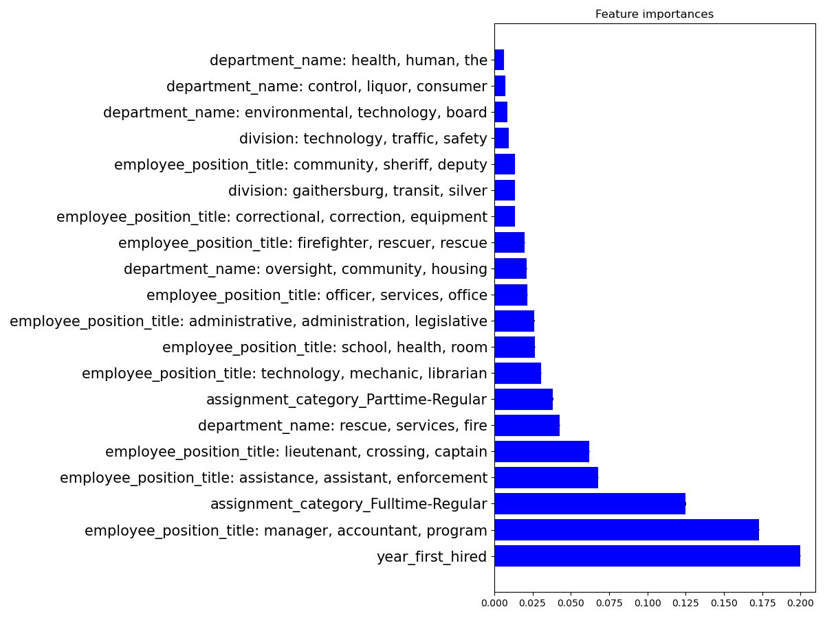
Feature importance in the statistical model
Here we consider interpretability, plot the feature importances of a
classifier. We can do this because the GapEncoder leads to
interpretable features even with messy categories
First, let’s train the RandomForestRegressor,
from sklearn.ensemble import RandomForestRegressor
regressor = RandomForestRegressor()
regressor.fit(X_train_enc, y_train)
Retrieving the feature importances
importances = regressor.feature_importances_
std = np.std(
    [
        tree.feature_importances_
        for tree in regressor.estimators_
    ],
    axis=0
)
indices = np.argsort(importances)[::-1]
Plotting the results:
import matplotlib.pyplot as plt
plt.figure(figsize=(12, 9))
plt.title("Feature importances")
n = 20
n_indices = indices[:n]
labels = np.array(feature_names)[n_indices]
plt.barh(range(n), importances[n_indices], color="b", yerr=std[n_indices])
plt.yticks(range(n), labels, size=15)
plt.tight_layout(pad=1)
plt.show()
We can deduce from this data that the three factors that define the most the salary are: being hired for a long time, being a manager, and having a permanent, full-time job :).
Exploring different machine-learning pipeline to encode the data
The learning pipeline
To build a learning pipeline, we need to assemble encoders for each column, and apply a supervised learning model on top.
Encoding the table
The TableVectorizer applies different transformations to the different columns to turn them into numerical values suitable for learning
from skrub import TableVectorizer
encoder = TableVectorizer()
Pipelining an encoder with a learner
Here again we use a pipeline with HistGradientBoostingRegressor
from sklearn.ensemble import HistGradientBoostingRegressor
pipeline = make_pipeline(encoder, HistGradientBoostingRegressor())
The pipeline can be readily applied to the dataframe for prediction
pipeline.fit(df, y)

# The categorical encoders
# ........................
#
# A encoder is needed to turn a categorical column into a numerical
# representation
from sklearn.preprocessing import OneHotEncoder

one_hot = OneHotEncoder(handle_unknown='ignore', sparse_output=False)
Dirty-category encoding
The one-hot encoder is actually not well suited to the ‘Employee Position Title’ column, as this columns contains 400 different entries.
We will now experiments with different encoders for dirty columns
from skrub import SimilarityEncoder, MinHashEncoder,\
    GapEncoder
from sklearn.preprocessing import TargetEncoder

similarity = SimilarityEncoder()
target = TargetEncoder()
minhash = MinHashEncoder(n_components=100)
gap = GapEncoder(n_components=100)

encoders = {
    'one-hot': one_hot,
    'similarity': similarity,
    'target': target,
    'minhash': minhash,
    'gap': gap}
We now loop over the different encoding methods, instantiate each time a new pipeline, fit it and store the returned cross-validation score:
all_scores = dict()

for name, method in encoders.items():
    encoder = TableVectorizer(high_cardinality=method)

    pipeline = make_pipeline(encoder, HistGradientBoostingRegressor())
    scores = cross_validate(pipeline, df, y)
    print('{} encoding'.format(name))
    print('r2 score:  mean: {:.3f}; std: {:.3f}'.format(
        np.mean(scores['test_score']), np.std(scores['test_score'])))
    print('time:  {:.3f}\n'.format(
        np.mean(scores['fit_time'])))
    all_scores[name] = scores['test_score']
one-hot encoding
r2 score:  mean: 0.790; std: 0.035
time:  2.968

similarity encoding
r2 score:  mean: 0.930; std: 0.011
time:  4.063

target encoding
r2 score:  mean: 0.906; std: 0.017
time:  0.407

minhash encoding
r2 score:  mean: 0.924; std: 0.012
time:  1.492

gap encoding
r2 score:  mean: 0.929; std: 0.013
time:  7.753
Note that the time it takes to fit varies also a lot, and not only the prediction score
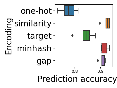
Plotting the results
Finally, we plot the scores on a boxplot:
import seaborn
import matplotlib.pyplot as plt
plt.figure(figsize=(4, 3))
ax = seaborn.boxplot(data=pd.DataFrame(all_scores), orient='h')
plt.ylabel('Encoding', size=20)
plt.xlabel('Prediction accuracy     ', size=20)
plt.yticks(size=20)
plt.tight_layout()
The clear trend is that encoders that use the string form of the category (similarity, minhash, and gap) perform better than those that discard it.
SimilarityEncoder is the best performer, but it is less scalable on big data than MinHashEncoder and GapEncoder. The most scalable encoder is the MinHashEncoder. GapEncoder, on the other hand, has the benefit that it provides interpretable features, as shown above
Total running time of the script: (2 minutes 14.831 seconds)